Throughout the 1990s,
the results of the NSS "thin samples" on household consumption
expenditure generated much interest in both academic and policy circles.
These results, which suggested at an all-India level that rural poverty
did not show any declining trend over the 1990s despite higher rates
of aggregate GDP growth, were seen as important inputs into the ongoing
policy debate on the effects of the liberalising economic policies instituted
by successive governments over the 1990s.
Those who had been questioning
the economic reform package have pointed out that these policies have
led to a neglect of rural and agricultural investment, resulting in
reduced productive employment opportunities in rural areas and to higher
food prices, developments likely to be associated with persistent or
even increasing rural poverty. They pointed out that the evidence of
stagnation or even decline in rural non-agricultural employment was
also in conformity with the evidence of persisting rural poverty.
By contrast, proponents of the
economic policies of the 1990s suggested that the "thin samples"
simply did not allow for such conclusions, and that nothing could be
said about rural consumption or poverty until the next large sample
results were available. It was also argued by proponents of the official
economic reform strategy, that the NSS consumption expenditure estimates
from the thin samples were out of sync with the CSO estimates of GDP.
Thus they maintained that the association of higher GDP growth rates
with the persistence of rural poverty in particular was not a real fact
which needed to be understood and addressed, but more of a failure of
the statistical system to capture the actual consumption in rural areas.
With this background, obviously
the results of the 55th Round (1999-2000) of the NSS, which is the first
"large sample" since 1993-94, have been eagerly awaited. Now
that the round is complete and the data due to be released later this
year, it has also become evident that this NSS Round is important and
interesting for another reason. This is that in the 55th Round, a different
technique has been used to establish household consumption levels. The
basic change is in terms of a change in the reference period.
Since the 1950s, the NSS consumption
surveys have been using an uniform reference period of one month. Since
the interviews are evenly spread out over the year, problems of seasonality
were ironed out. However, in recent years the NSS has revived the issue
of whether a one week reference period is more suitable for determining
non-durable consumption than the one month reference period currently
used.
This is not a new issue : indeed,
it is a question which has been of concern to the NSS since the very
inception of the surveys in the early 1950s. In fact, in the formative
years of the NSS, considerable attention was paid to the length of reference
period suitable for ascertaining the correct level of consumption of
different items of goods and services, and a special report was brought
out covering the period April 1951 to March 1954 on the suitability
of reference period.
Most interestingly, the NSS under
guidance of P.C. Mahalanobis had carried out a special investigation
into this very issue in March-April 1952, based on 1254 households of
76 villages of West Bengal. The households were divided into two groups.
For one group, consumption details were procured by actual weighing
of food items (clean rice, pulses, sugar and salt) by field staff. For
the other group, data collection was by questioning, and here again
the group was divided equally between those for whom the questions pertained
to a reference period of one week and those for whom the reference period
was one month.
The results were quite interesting.
It was found that the two sets of data obtained by questioning differed
quite sharply, with the consumption estimates obtained on the basis
of the one week reference period being much higher than those obtained
on the basis of one month recall. It was also found that the one month
reference period generated information that corresponded much more closely
to the data on the basis of actual weighing of food items. This led
Mahalanobis and others to conclude that the one month reference period
was better suited to the purposes of the estimates especially of food
consumption.
Since then, it has been standard
for the National Sample Survey to use the one month reference period
for food items, although both the one month and one year reference period
have been used for some non-food items. In the five quinquennial surveys
of household consumption expenditure between 1972-73 and 1993-94, information
for clothing, footwear and durable goods was collected from each sample
household for two reference periods - "last 30 days" and "last
365 days". In the 50th round, "educational" and "institutional
medical" expenses were also added to the list of items for which
data were collected by these two reference periods.
However, during the 1990s, the
question of the most suitable reference period has resurfaced, and the
NSS has in its thin samples experimented on the basis of alternative
schedules (based on one week and one month recall) in independent samples
during the course of the same survey. This was done for the 51st Round
(1994-95), the 52nd Round (1995-96), the 53rd Round (1997) and the 54th
Round (Jan-Jun 1998).
In all of these surveys, half
the sample was canvassed using a Type 1 schedule which had a 30 day
reference period for all items, but the other half was canvassed using
a Type 2 schedule which had a one week reference period for food, pan,
tobacco and intoxicants and a one year reference period for clothing,
footwear, durable goods and educational and medical (institutional)
services. However, since the Type 2 schedule was not comparable to earlier
NSS surveys, the results by this schedule were not tabulated in the
NSS Reports of the relevant rounds, so that all the available analysis
of consumer expenditure and of poverty during the nineties are based
on the Type 1 schedule.
It is now reported that for the
large sample of 1999-2000, this experiment has been carried one step
further, to the point where the two different schedules of Type 1 (one
month) and Type 2 (one week) have been canvassed from every sample household.
To the extent that the two schedules give varying results, incorporating
them so that all the households respond to both schedules is obviously
problematic since it would bias the results of both schedules. It also
means that there are definite problems of comparability with data from
past surveys, for which the reference period was essentially one month
and one week was not used at all.
Fortunately, the NSS has now
released the preliminary results on the effect of the choice of reference
period for the 51st, 52nd, 53rd and 54th Rounds in its Report No. 447:
Choice of Reference Period for Consumption Data. It is, therefore, possible
to examine the effect of choosing one reference period over another.
As mentioned, above, in all of these Rounds, one half of the sample
(Type 1) had a reference period of one month (30 days) throughout; for
the other half (Type 2) the reference periods were as follows : one
week for all food, pan, tobacco and intoxicants; one month for fuel
and light and miscellaneous goods and services; and one year for clothing,
footwear and durable goods as well as education and institutional medical
expenses.
The results of these samples
based on alternative schedules are extremely interesting. It emerges
that Type 2 samples give higher overall food consumption, exactly as
Mahalanobis had predicted and as was also confirmed by the pilot investigation
in the West Bengal villages in 1952. Thus, the Type 2 schedule-based
samples also suggest that poverty is much lower.
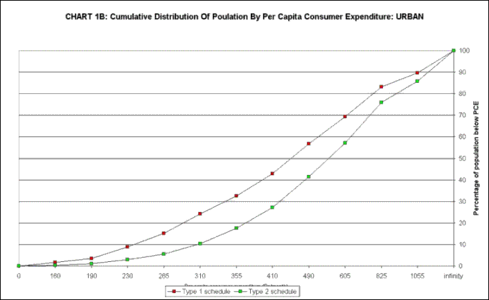
In Charts 1A and 1B, the cumulative distribution of population below
specified per capita total consumption levels as obtained from the Type
1 and Type 2 schedules are plotted for the rural and urban sectors,
using data from the 52nd round. It may be seen that the proportion of
population below any expenditure level is always higher by the Type 1
schedule than by Type 2, and the difference is extremely large. Thus,
using the Planning Commission poverty line, about 39 per cent of the
rural population would be below the poverty line in 1995-96 by the Type
1 schedule but this percentage would be only around 20 per cent by the
Type 2 schedule. The corresponding percentages for urban areas are 30
and 15. Similarly large differences are obtained for the 51st, 53rd and
54th rounds.

This of course raises the question
about which of these two schedules gives a better measure of the actual
incidence of poverty in India. But an even more important problem is
the implication that the 55th round may end up giving a totally biased
picture of poverty trends during the 1990s if the results from this
are compared to earlier rounds which did not use the "one week"
reference period.
Thus, suppose, for example, the
55th Round comes up with an estimate of 25 per cent of rural population
below the poverty line in 1999-2000. This would be compared to the corresponding
37 percent rural poverty obtained from the 50th Round in 1993-94, and
the implied large reduction in poverty would be greeted by the reformers
as vindication of their policies. But, since this does not compare like
with like, such a conclusion would obviously be erroneous and the debate
about trends in poverty would enter a statistical minefield which the
55th Round results will not be able to resolve.
The problem is that since the
55th Round has canvassed both the Type 1 and Type 2 schedules from all
households, there would have been a pressure for consistency between
the answers to the "one week" and "one month" reference
periods on the part of both respondents and investigators. It is obvious
that when the household is questioned using both the one week and one
month reference period, the answers are likely to be tested by simple
multiplication of the one week reply for the monthly response as well.
This means that the two schedules can no longer be seen as independent
and may give misleading results depending upon how the conflation of
the referenced periods affects the responses.
If such pressure for consistency
has led to primacy being given to the "one week" response,
a 25 per cent rural poverty incidence in the 55th round would correspond
to a 45 per cent poverty incidence by the procedure followed in 1993-94
so that the proponents of liberalising reforms could end up claiming
massive poverty reduction while in fact poverty might have increased
massively.
Even if the pressure for consistency
has worked evenly across the schedules, so that the 55th Round results
are an average of the two, a 25 per cent rural poverty incidence in
this Round would correspond to a 36 per cent poverty by the method used
in earlier rounds, so that a large poverty reduction could be claimed
without there having been any significant reduction from the actual
poverty level in 1993-94.
In view of this, the 55th Round
stands severely compromised in its ability to give estimates of mean
consumer expenditure and poverty comparable to that in earlier Rounds.
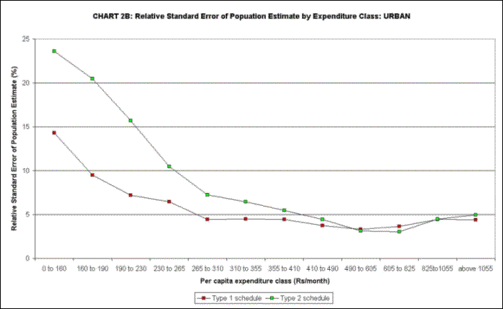
This is particularly the case because, as Charts 2A and 2B show, the
errors associated with measuring the population in lower expenditure
classes is much higher by the Type 2 schedule. These errors are computed
by the NSSO on the basis of the variance obtained across sub-samples
in the same survey and for the same schedule type, and show the much
greater inherent unreliability of poverty estimates calculated with
data from the Type 2 schedule.

The National Sample Survey Organisation
needs, therefore, to conduct another large sample survey on the basis
of the earlier schedule exclusively, to give comparable estimates. In
the meantime, the 55th Round should be treated as an experimental survey
whose comparability with past surveys is poor, but which may further
elucidate the intriguing differences revealed by the results of the
51st to 54th Round surveys. This is important because much mud has been
slung at the NSS consumer expenditure data in the course of the recent
debate on poverty, and the air needs to be cleared so that questions
about the reliability of data does not continue to cloud assessment
of such an important issue.
Much of the criticism of NSS
data in the recent past has concentrated on the fact that these give
lower estimates of total consumer expenditure than the alternative estimates
from the National Accounts Statistics (NAS), and some have even claimed
that the difference between these two estimates have grown alarmingly
during the nineties. In an earlier edition of Macroscan (February 22nd,
2000), it had been pointed out that although the NSS does indeed give
a lower estimate of overall consumption than the NAS, and although the
difference did increase during the seventies and eighties, the ratio
between these two estimates have remained fairly stable during the nineties
so that the 1990s trends in poverty obtained from NSS data cannot be
challenged on this ground.
Nonetheless, since this has been
the main thrust of the attack on the NSS data so far, we present in
Table 1 the ratios of the NSS to NAS estimates of consumption by broad
items and over successive full-year NSS rounds beginning 1977-78. Since
only the NAS estimates with base 1980-81 cover this entire period, these
ratios have been calculated with these NAS estimates rather than the
new estimates with 1993-94 as base. As mentioned earlier, the ratio
of total NSS consumption to NAS consumption is seen to decline from
0.81 in 1977-78 to 0.69 in 1990-91 but remains almost constant thereafter.
However, the more important differences between these two estimates
relate to the item-wise results.
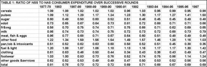
As may be seen there are certain
persistent differences between these two data sets at the level of individual
items. Thus, for sugar, edible oils, fruits & vegetables, milk &
products, pan, tobacco & intoxicants, and other goods & services,
the NSS has consistently measured lower consumption but with no obvious
time trend in these ratios. In the case of meat,fish & eggs and
clothing, NSS has lower consumption and the ratio has fallen over time.
For cereals, the ratio has always been close to unity but with some
tendency to decline over time. But, for pulses, other food and fuel
& light, the NSS has consistently measured higher consumption than
the NAS.
These persistent differences
between NSS and NAS data have been analysed thoroughly by resarchers,
notably B.S. Minhas and his associates, who have noted that it is normal
all over the world for items like intoxicants to be under-reported by
respondents and that something similar is probably true also for non-vegetarian
items in a country such as India.
Also, they note that much of
sugar, edible oils, milk & products and fruit & vegetables are
consumed not directly by households but are purchased after processing
either by hotels and restaurants or by other manufacturers. In such
cases, these would appear differently in the NSS and NAS data, with
the former including these under "other foods" while the latter
would include them directly under the item concerned.
This explains also why the NSS
has tended to measure higher expenditure under "other food".
The relative over-estimation by the NSS of fuel & light has likewise
been explained by failure of the NAS to adequately capture fuel wood
and twigs collected directly by households. Thus, for most of the above
items, the differences are not particularly surprising or unexpected,
especially given that the NSS does not capture all consumer expenditure
since it leaves out institutional consumption such as in hostels, prisons
and ceremonials.
However, for certain items such
as clothing and "other non-food" the differences are large
and have been attributed in past analysis both to a failure of NAS to
measure household consumption correctly and to a failure of the NSS
to adequately capture the consumption of the relatively richer household
who consume relatively more of these.
Indeed, it is on the basis of
the these observations, that the Expert Group on Poverty Estimates had
decided in 1993 that the differences between the NSS and NAS were unlikely
to cause any serious bias in poverty measures estimated directly from
NSS estimates, and had accordingly decided to end the practice till
then of adjusting these estimates to conform to the NAS.
However, the issue of alternative
reference periods has now again opened up this issue since apparently
much of the difference in food consumption between the NAS and the NSS
can be resolved if the one week rather than the one month schedule is
used in the latter. Indeed, in its Report No. 477, the NSSO reports
higher errors for week-based estimates as compared to estimates based
on 30 days, but on noting that "the substantial and systematic
differences between the week and month based estimates indicate that
one or both methods are not depicting the real life situation",
goes on to claim some support for the Type 2 schedule since the total
of the one week estimates is closer to the NAS than the totals of the
30 day estimates.
Although the NSSO itself is careful
on the matter, suggesting that further methodological surveys would
be advisable, others may not be so careful. They may not only ignore
the fact that the relative standard error of each item canvassed on
the one week basis is higher than by the 30 day schedule, but also fail
to notice that the recent experiments merely reproduce what Mahalanobis
and his associates had found almost 50 years ago.
As mentioned earlier, it was
found in the 1950s that the one month estimate of most food items was
lower than the one week estimate but was in greater conformity with
the physical (weight) measures of actual household consumption of foodstuffs,
than the one week estimate. Thus, the bias between results from the
two reference periods continues to remain in the same direction, and
with no experiment through physical weighment repeated, there is no
further evidence for judging the relative plausibility of the two estimates.
Comparison with NAS is a poor substitute given the past judgement of
researchers such as Minhas and the assessment of the Expert Group on
Poverty Estimates, both of which found strong reason not to accept the
NAS as necessarily giving reliable estimates.
Table 2 gives the perentage differences
between the NSS and NAS (1980-81) using both the schedules in the former.
It may be noticed that although the Type 2 NSS estimates are fairly
close to the NAS for all food items taken together, while the Type 1
NSS estimates are about 20 per cent lower, this result comes about because
the Type 2 estimate gives higher estimates for all food items including
for those where the Type 1 estimate is higher than the NAS estimate.
As a consequence, the apparent concordance between the Type 2 NSS estimates
and the NAS is something of statistical artifact because these week-based
results continue to show large shortfalls from the corresponding NAS
estimates for sugar, edible oils, milk & products and meat, fish
& eggs but almost double the estimate for "other food".
If both positive and negative divergence are given equal weight to measure
the difference between the NSS and NAS, the results from the Type 1
schedule turn out to be closer to the NAS for food items. Also the large
gap between the NAS and NSS for non-food is further widened when the
Type 2 rather than the Type 1 results are considered.
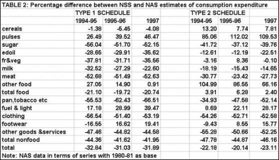
Table 3 gives the absolute value of consumption estimates for 1995-96 from both the Type 1 and Type 2 NSS schedules and from both the NAS estimates with base 1980-81 and base 1993-94. This not only shows the patterns discussed above but also certain inherent infirmities in the NAS data.
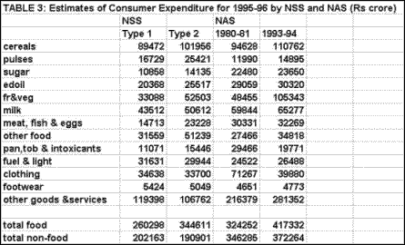
Thus, for two items, "pan,
tobacco and intoxicants" and "clothing", the NAS has
substantially revised downwards its consumption estimates, between the
1980-81 and 1993-94 series, bringing these closer to the NSS estimates.
But for two others, "fruits and vegetables" and "other
non-food" the NAS has revised upwards its estimates and thus increased
the gap with the NSS. For "other non-food" there is at least
the likelihood that new goods and services were being underestimated
earlier and may not be captured in the NSS which does miss out on the
rich who consume these more, but the doubling of fruit and vegetable
consumption is intriguing and highly suspicious.
As discussed in an earlier Macroscan,
not only does this not correspond with the known area under horticultural
crops, it has the effect of making the NAS estimate three times the
NSS Type 1 estimate and more than double even the NSS Type 2 estimate.
In view of these large and sometimes inexplicable revisions, the NAS
can hardly be said to represent the type of benchmark that Mahalanobis
had set himself when he actually carried out physical weighment to
check the validity of reference periods.
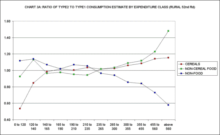
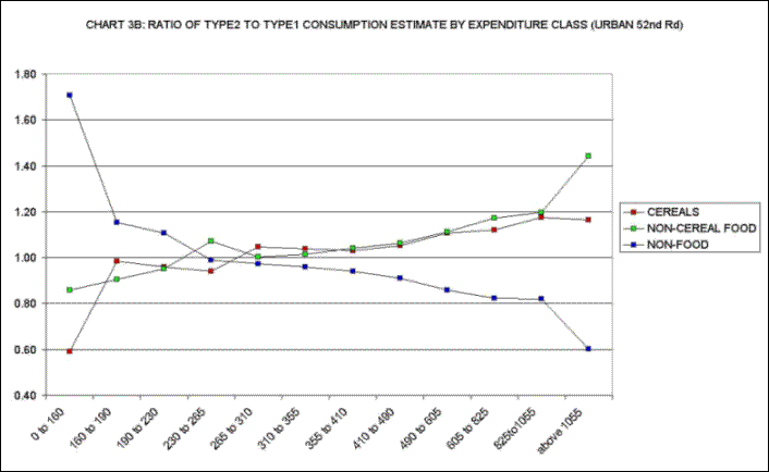
Finally, as Charts 3A and 3B
show, there is the intriguing fact that the Type 2 schedule sample results
show richer households consuming relatively more food and less non-food
as compared to the Type 1 schedule, thus overturning much of what is
now accepted wisdom regarding changing consumption habits along the
Engels Curve. This too should suggest a more careful look at the estimates
emanating from the Type 2 schedules, and by implication, of the overall
consumption results of the 55th Round.